11 Mapping SNPs onto 3D Protein Structures with Chimera and AlphaFold

12 Overview
In this module you will learn how to:
- Retrieve AlphaFold protein structures
- Prepare residue-level SNP attribute files for Chimera
- Map SNP counts onto a 3D structure in UCSF Chimera
- Interpret mutation density in structural context
We use the Mycobacterium tuberculosis protein Rv3872 (PE35) as a worked example.
12.1 Learning goals
By the end you should be able to:
- Generate a valid Chimera attribute file (.defattr) from a residue-level SNP table
- Load the attribute into Chimera and color a structure by SNP burden
- Compare cartoons, side chains and surfaces to localize hotspots
- Combine SNP burden with AlphaFold confidence to avoid over-interpreting low-confidence regions
12.2 Inputs for this practical
AlphaFold model (example):
Example residue-level SNP count table (text):
An example of a problematic CSV format (comma separated):
13 Background
Mapping SNPs onto protein structures can help you identify mutation hotspots, assess structural clustering and generate mechanistic hypotheses. It is most informative when combined with: variant effect type, lineage context, phenotypes such as MIC, and structural confidence from AlphaFold.
This practical focuses on the mechanics of getting from a residue-level SNP table to a useful structural visualization.
14 Step 1: Obtain a structure
- Open AlphaFold DB
- Search for the UniProt ID of the protein of interest (for Rv3872: P9WIG7)
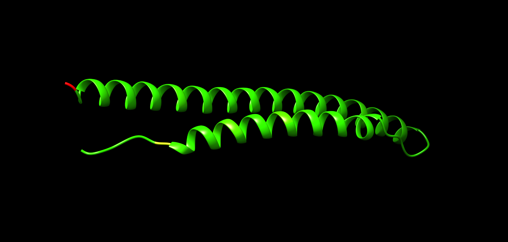
- Download the structure, ideally as mmCIF. PDB also works.
If you already have an AlphaFold PDB file, you can proceed directly.
Figure examples below show the same structure in different representations you will recreate in Chimera.
15 Step 2: Prepare an attribute file for Chimera
Chimera can color residues by a custom attribute. The attribute is supplied as a plain text file with a required header and one line per residue.
A minimal .defattr structure is:
attribute: nsSNPs
match mode: 1-to-1
recipient: residues
    :1    0
    :2    0
    :3    0
15.1 Key rules to avoid failure
- Use tabs between the residue selector and the value
- Residue numbering must match the model residue numbering
- Remove STOP codon or any non-residue entries
- Do not use commas as separators
Tip: validating a .defattr file quickly
Open the file in a plain text editor and confirm:
- The first three header lines exist exactly once
- Data lines start with a colon, then a residue number
- Columns are separated by a tab, not spaces or commas
15.2 Automating attribute creation
You can generate a .defattr from a two-column table residue,count. Below are two options: a small Python script and an awk one-liner. Both avoid manual spreadsheet editing.
Option A: Python script ^^^^^^^^^^^^^^^^^^^^^^^
Save as make_defattr.py and run from the command line.
import argparse
import csv
import sys

def read_table(path, delimiter):
    rows = []
    with open(path, "r", newline="", encoding="utf-8") as handle:
        reader = csv.reader(handle, delimiter=delimiter)
        for row in reader:
            if not row:
                continue
            if len(row) < 2:
                continue
            a, b = row[0].strip(), row[1].strip()
            if not a or not b:
                continue
            if not a.isdigit():
                continue
            try:
                val = float(b)
            except ValueError:
                continue
            rows.append((int(a), val))
    return rows

def main():
    ap = argparse.ArgumentParser()
    ap.add_argument("--infile", required=True)
    ap.add_argument("--outfile", required=True)
    ap.add_argument("--attribute", default="nsSNPs")
    ap.add_argument("--delimiter", default="\t")
    ap.add_argument("--drop-residues", default="")
    args = ap.parse_args()

    delimiter = args.delimiter.encode("utf-8").decode("unicode_escape")
    rows = read_table(args.infile, delimiter)

    drop = set()
    if args.drop_residues.strip():
        for x in args.drop_residues.split(","):
            x = x.strip()
            if x.isdigit():
                drop.add(int(x))

    rows = [(r, v) for r, v in rows if r not in drop]
    rows.sort(key=lambda t: t[0])

    with open(args.outfile, "w", encoding="utf-8") as out:
        out.write(f"attribute: {args.attribute}\n")
        out.write("match mode: 1-to-1\n")
        out.write("recipient: residues\n")
        for r, v in rows:
            if v.is_integer():
                vtxt = str(int(v))
            else:
                vtxt = str(v)
            out.write(f"\t:{r}\t{vtxt}\n")

if __name__ == "__main__":
    main()
Example runs:
python make_defattr.py --infile Rv3872_SNPcount_two_col.tsv --outfile Rv3872_nsSNPs.defattr
python make_defattr.py --infile NOTgoodComma.csv --delimiter "," --outfile Rv3872_nsSNPs.defattr
Option B: awk one-liner ^^^^^^^^^^^^^^^^^^^^^^^
Works when your input is already two columns residue tab count.
awk 'BEGIN{print "attribute: nsSNPs"; print "match mode: 1-to-1"; print "recipient: residues"} {if ($1 ~ /^[0-9]+$/) print "\t:"$1"\t"$2}' input.tsv > Rv3872_nsSNPs.defattr16 Step 3: Open the model in Chimera
Install and open UCSF Chimera.
- File → Open → select your model file (.pdb or .cif)
Recommended initial view setup:
- Actions → Ribbon → show
- Presets → Interactive 1 (optional)
17 Step 4: Load the residue attribute and color the structure
17.1 Define the attribute
- Tools → Structure Analysis → Define Attribute
- Load your .defattr file
- Confirm recipient is residues and the attribute name is nsSNPs
17.2 Render by attribute
- Tools → Structure Analysis → Render by Attribute
- Attribute: nsSNPs
- Recipient: residues
- Choose a color ramp and adjust thresholds
You should now see high-burden residues highlighted.
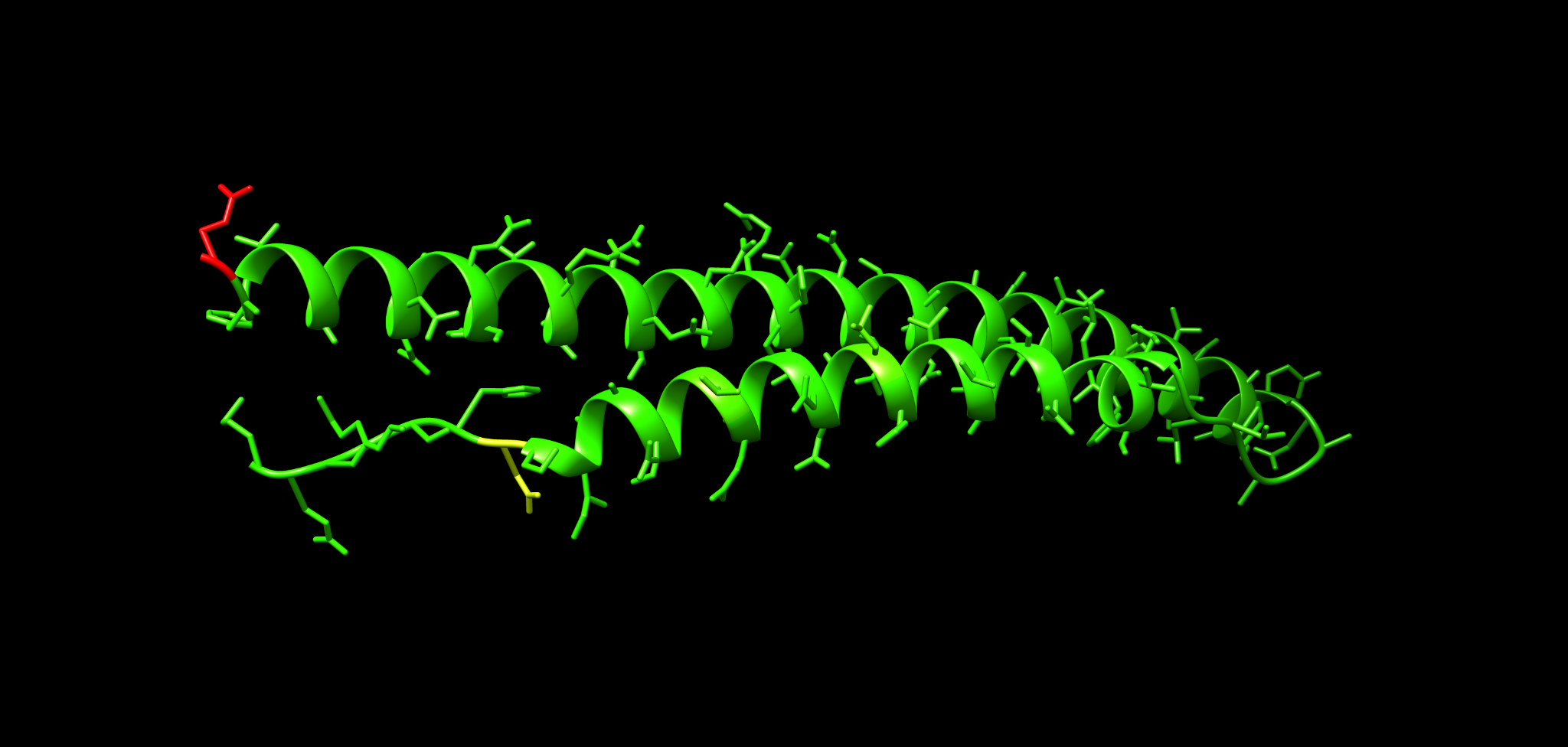
Example representation with side chains shown:
18 Step 5: Switch representations to interpret the pattern
18.1 Cartoon plus side chains
Use this to see whether hotspots fall on particular helices or loops.
- Actions → Atoms/Bonds → show
- Actions → Atoms/Bonds → stick (optional for emphasis)
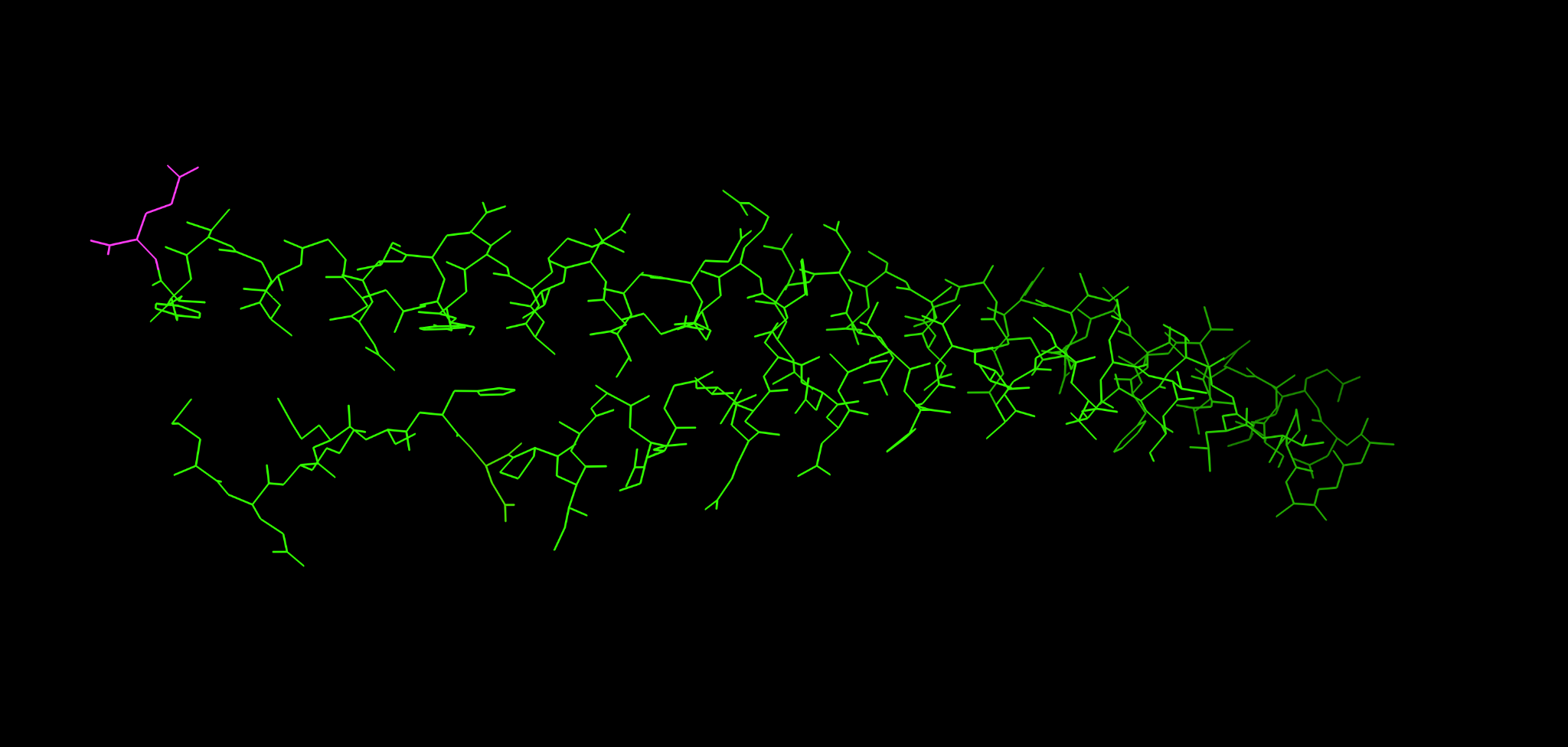
18.2 Wire or stick emphasis
This view is useful when you want the mutation pattern to stand out from the backbone.
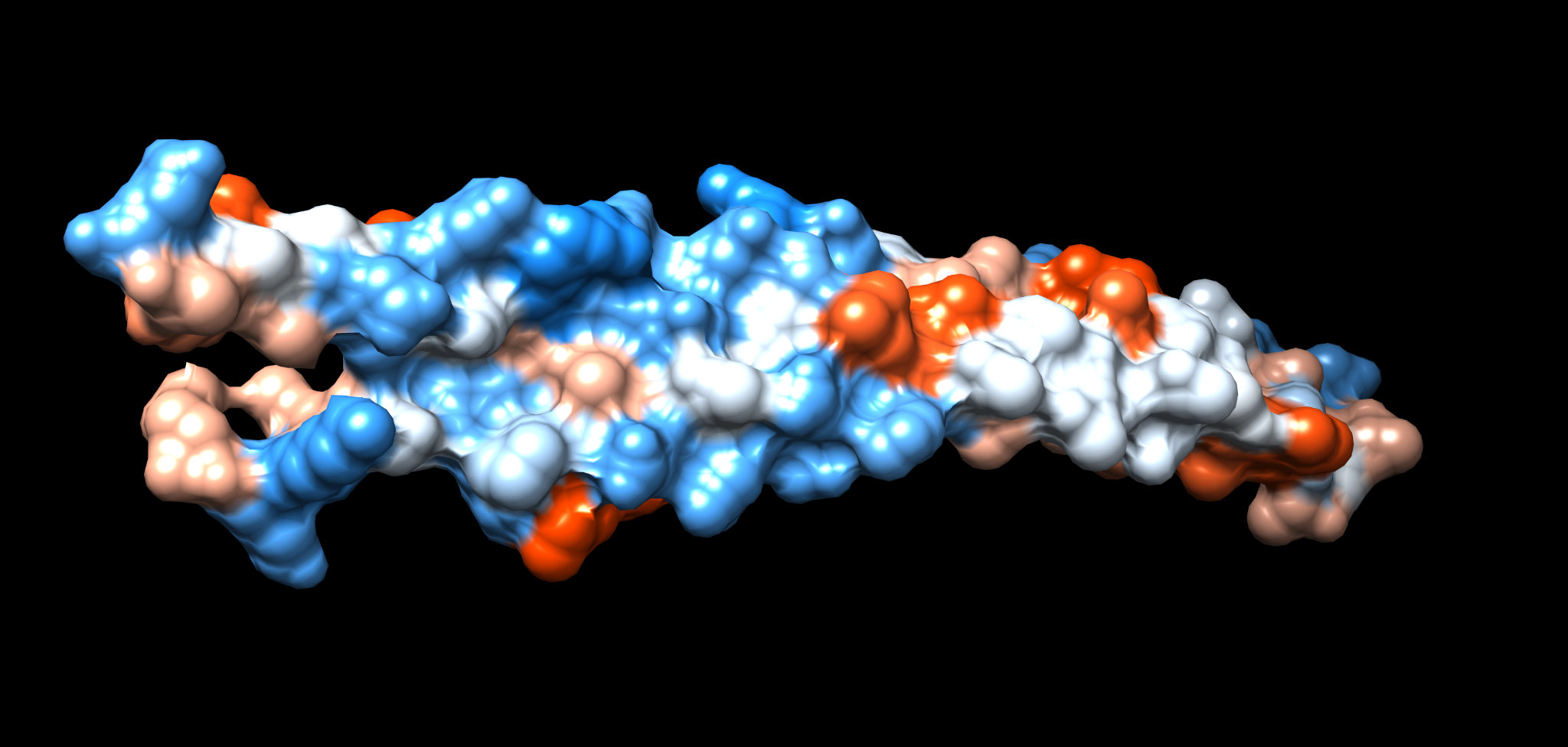
18.3 Surface view
Surfaces help decide whether hotspots are likely exposed.
- Actions → Surface → show
- Tools → Depiction → Surface (optional refinements)
Electrostatics are often inspected alongside SNP burden when you suspect interaction interfaces.
19 Step 6: Add AlphaFold confidence as a sanity check
AlphaFold structures include per-residue confidence (pLDDT). A common pitfall is to interpret clustering in regions with low confidence, often flexible or disordered.
Practical guidance:
- Treat high SNP density in low-confidence segments as weak structural evidence
- Prefer conclusions from regions with consistently high confidence
In Chimera you can inspect confidence if it is stored as a B-factor like field in your model, depending on file type. If not available, obtain confidence from the AlphaFold download and map it as a second attribute using the same mechanism as for nsSNPs.
20 Exercises
Load the Rv3872 structure, load your nsSNPs attribute and color the structure by SNP count.
Answer briefly:
- Which residue index has the highest SNP count in your table
- Is it located in a helix or in a loop
- Does it appear surface exposed in the surface view
Adjust the color thresholds so that:
- 0 to 5 is low burden
- 5 to 20 is medium burden
- greater than 20 is high burden
Does the hotspot pattern become easier to interpret or does it become misleading
Overlay or separately color by confidence and decide which parts of the protein you trust structurally.
List one region you would prioritize for follow-up and one region you would treat cautiously.
21 Common troubleshooting
Attribute file loads but nothing changes:
- Check that residue numbering matches the model
- Confirm match mode 1-to-1
- Confirm recipient residues
- Confirm tabs are present
Chimera errors on load:
- Remove non-residue lines, especially STOP codon entries
- Remove commas and ensure tab separation
Hotspot appears in an unstructured tail:
- Check AlphaFold confidence and avoid over-interpreting low-confidence segments
22 Further reading and resources
- Chimera tutorials: https://www.cgl.ucsf.edu/chimera/tutorials.html
- Chimera getting started: https://www.cgl.ucsf.edu/Outreach/Tutorials/GettingStarted.html
- Protein structure analysis course: https://elearning.vib.be/courses/protein-structure-analysis/lessons/introduction/topic/sequences-and-structures/